Chapter 3: Radio Transmission

For anyone familiar with wireless access technologies that offer a best-effort service, such as Wi-Fi, the cellular network presents a notable contrast. This is mostly because cellular networks carefully allocate available radio spectrum among many users (or more precisely, UEs), aiming to deliver a certain quality to all active users in a coverage area, while also allowing those users to remain connected while moving. They also aim to maximize the efficiency of spectrum usage, as it is a finite and often costly resource. This has resulted in a highly dynamic and adaptive approach, in which coding, modulation and scheduling play a central role. 5G takes the cellular approach to managing radio resources to a new level of sophistication.

Wireless transmission is full of challenges that don’t arise in wired networks. Interference can arise from many sources ranging from microwave ovens to baby monitors, while radio signals reflect off objects such as buildings and vehicles. Some objects absorb wireless signals. The properties of the wireless channel vary over time, and depending on the frequency in use. Much of the design of cellular radio systems is motivated by the need to deal with these challenges.

As we will see in this chapter, mobile cellular networks use a reservation-based strategy, whereas Wi-Fi is contention-based. This difference is rooted in each system’s fundamental assumption about utilization: Wi-Fi assumes a lightly loaded network (and hence optimistically transmits when the wireless link is idle and backs off if contention is detected), while 5G assumes (and strives for) high utilization (and hence explicitly assign different users to different “shares” of the available radio spectrum).

The fact that 5G controls spectrum allocation carefully is central to its ability to deliver guarantees of bandwidth and latency more predictably than Wi-Fi. This in turn is why there is so much interest in using 5G for mission-critical applications.

We start by giving a short primer on radio transmission as a way of laying a foundation for understanding the rest of the 5G architecture. The following is not a substitute for a theoretical treatment of the topic, but is instead intended as a way of grounding the systems-oriented description of 5G that follows in the reality of wireless communication.

3.1 Coding and Modulation

The mobile channel over which digital data needs to be reliably transmitted brings a number of impairments, including noise, attenuation, distortion, fading, and interference. This challenge is addressed by a combination of coding and modulation, as depicted in Figure 17.

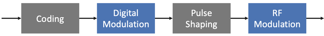
Figure 17. The role of coding and modulation in mobile communication.

At its core, coding inserts extra bits into the data to help recover from all the environmental factors that interfere with signal propagation. This typically implies some form of Forward Error Correction (e.g., turbo codes, polar codes). Modulation then generates signals that represent the encoded data stream, and it does so in a way that matches the channel characteristics: It first uses a digital modulation signal format that maximizes the number of reliably transmitted bits every second based on the specifics of the observed channel impairments; it next matches the transmission bandwidth to channel bandwidth using pulse shaping; and finally, it uses RF modulation to transmit the signal as an electromagnetic wave over an assigned carrier frequency.

For a deeper appreciation of the challenges of reliably transmitting data by propagating radio signals through the air, consider the scenario depicted in Figure 18, where the signal bounces off various stationary and moving objects, following multiple paths from the transmitter to the receiver, who may also be moving.

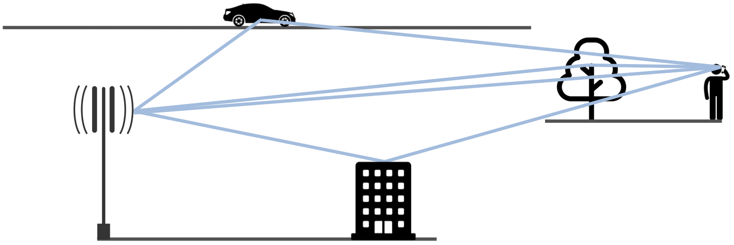
Figure 18. Signals propagate along multiple paths from transmitter to receiver.

As a consequence of these multiple paths, the original signal arrives at the receiver spread over time, as illustrated in Figure 19. Empirical evidence shows that the Multipath Spread—the time between the first and last signals of one transmission arriving at the receiver—is 1-10μs in urban environments and 10-30μs in suburban environments. These multipath signals can interfere with each other constructively or destructively, and this will vary over time. Theoretical bounds for the time duration for which the channel may be assumed to be invariant, known as the Coherence Time and denoted \(T_c\), is given by

\[T_c =c/v \times 1/f\]

where \(c\) is the velocity of the signal, \(v\) is the velocity of the receiver (e.g., moving car or train), and \(f\) is the frequency of the carrier signal that is being modulated. This says the coherence time is inversely proportional to the frequency of the signal and the speed of movement, which makes intuitive sense: The higher the frequency (narrower the wave) the shorter the coherence time, and likewise, the faster the receiver is moving the shorter the coherence time. Based on the target parameters to this model (selected according to the target physical environment), it is possible to calculate \(T_c\), which in turn bounds the rate at which symbols can be transmitted without undue risk of interference. The dynamic nature of the wireless channel is a central challenge to address in the cellular network.

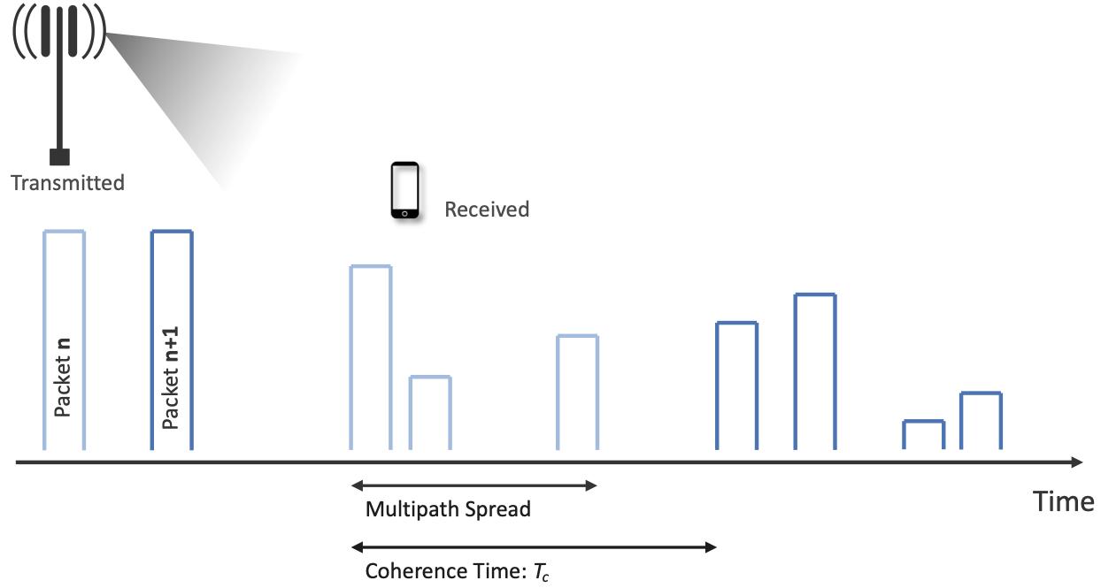
Figure 19. Received data spread over time due to multipath variation.

To complicate matters further, Figure 18 and 19 imply the transmission originates from a single antenna, but cell towers are equipped with an array of antennas, each transmitting in a different (but overlapping) direction. This technology, called Multiple-Input-Multiple-Output (MIMO), opens the door to purposely transmitting data from multiple antennas in an effort to reach the receiver, adding even more paths to the environment-imposed multipath propagation.

One of the most important consequences of these factors is that the transmitter must receive feedback from every receiver to judge how to best utilize the wireless medium on their behalf. 3GPP specifies a Channel Quality Indicator (CQI) for this purpose. In practice, the receiver sends a CQI status report to the base station periodically (e.g., every millisecond). These CQI messages report the observed signal-to-noise ratio, which impacts the receiver’s ability to recover the data bits. The base station then uses this information to adapt how it allocates the available radio spectrum to the subscribers it is serving, as well as which coding and modulation scheme to employ. All of these decisions are made by the scheduler.

3.2 Scheduler

How the scheduler does its job is one of the most important properties of each generation of the cellular network, which in turn depends on the multiplexing mechanism. For example, 2G used Time Division Multiple Access (TDMA) and 3G used Code Division Multiple Access (CDMA). How data is multiplexed is also a major differentiator for 4G and 5G, completing the transition from the cellular network being fundamentally circuit-switched to fundamentally packet-switched.

Both 4G and 5G are based on Orthogonal Frequency-Division Multiplexing (OFDM), an approach that multiplexes data over multiple orthogonal subcarrier frequencies, each of which is modulated independently. One attraction of OFDM is that, by splitting the frequency band into subcarriers, it can send symbols on each subcarrier at a relatively low rate. This makes it easier to correctly decode symbols in the presence of multipath interference. The efficiency of OFDM depends on the selection of subcarrier frequencies so as to avoid interference, that is, how it achieves orthogonality. That topic is beyond the scope of this book.

As long as you understand that OFDM uses a set of subcarriers, with symbols (each of which contain a few bits of data) being sent at some rate on each subcarrier, that you can appreciate that there are discrete schedulable units of the radio spectrum. The fundamental unit is the time to transmit one symbol on one subcarrier. With that building block in mind, we are now in a position to examine how multiplexing and scheduling work in 4G and 5G.

3.2.1 Multiplexing in 4G

We start with 4G because it provides a foundational understanding that makes 5G easier to explain, where both 4G and 5G use an approach to multiplexing called Orthogonal Frequency-Division Multiple Access (OFDMA). You can think of OFDMA as a specific application of OFDM. In the 4G case, OFDMA multiplexes data over a set of 12 orthogonal (non-interfering) subcarrier frequencies, each of which is modulated independently.1 The “Multiple Access” in OFDMA implies that data can simultaneously be sent on behalf of multiple users, each on a different subcarrier frequency and for a different duration of time. The 4G-defined subbands are narrow (e.g., 15 kHz), and the coding of user data into OFDMA symbols is designed to minimize the risk of data loss due to interference.

1

4G uses OFDMA for downstream traffic, and a different multiplexing strategy for upstream transmissions (from user devices to base stations), but we do not describe it because the approach is not applicable to 5G.

The use of OFDMA naturally leads to conceptualizing the radio spectrum as a 2-D resource, as shown in Figure 20, with the subcarriers represented in the vertical dimension and the time to transmit symbols on each subcarrier represented in the horizontal dimension. The basic unit of transmission, called a Resource Element (RE), corresponds to a 15-kHz band around one subcarrier frequency and the time it takes to transmit one OFDMA symbol. The number of bits that can be encoded in each symbol depends on the modulation scheme in use. For example, using Quadrature Amplitude Modulation (QAM), 16-QAM yields 4 bits per symbol and 64-QAM yields 6 bits per symbol. The details of the modulation need not concern us here; the key point is that there is a degree of freedom to choose the modulation scheme based on the measured channel quality, sending more bits per symbol (and thus more bits per second) when the quality is high.

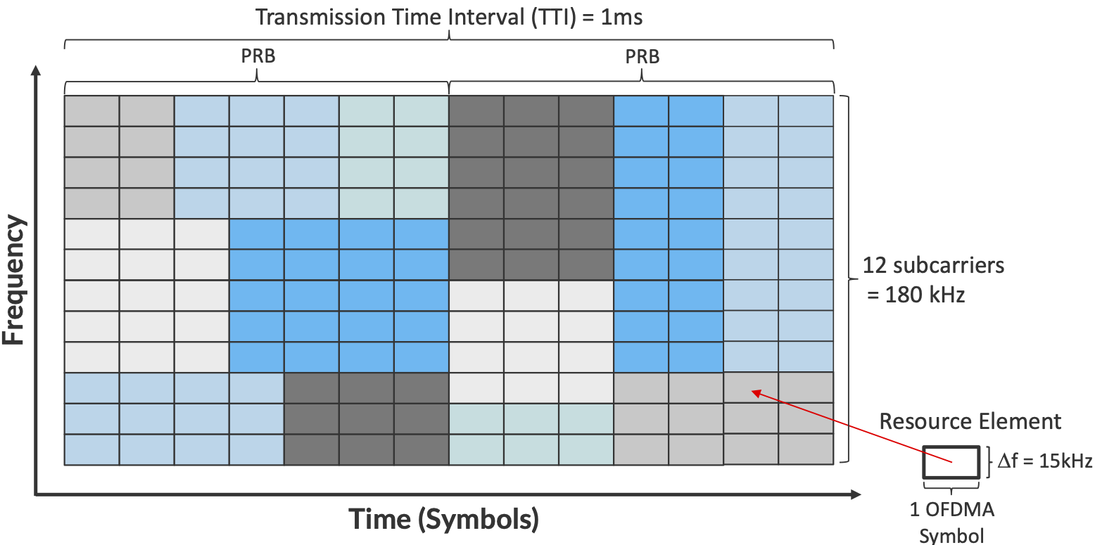
Figure 20. Spectrum abstractly represented by a 2-D grid of schedulable Resource Elements.

A scheduler allocates some number of REs to each user that has data to transmit during each 1 ms Transmission Time Interval (TTI), where users are depicted by different colored blocks in Figure 20. The only constraint on the scheduler is that it must make its allocation decisions on blocks of 7x12=84 resource elements, called a Physical Resource Block (PRB). Figure 20 shows two back-to-back PRBs. Of course time continues to flow along one axis, and depending on the size of the available frequency band (e.g., it might be 100 MHz wide), there may be many more subcarrier slots (and hence PRBs) available along the other axis, so the scheduler is essentially preparing and transmitting a sequence of PRBs.

Note that OFDMA is not a coding/modulation algorithm, but instead provides a framework for selecting a specific coding and modulation for each subcarrier frequency. QAM is one common example modulation. It is the scheduler’s responsibility to select the modulation to use for each PRB, based on the CQI feedback it has received. The scheduler also selects the coding on a per-PRB basis, for example, by how it sets the parameters to the turbo code algorithm.

The 1-ms TTI corresponds to the time frame in which the scheduler receives feedback from users about the quality of the signal they are experiencing. This is the role of CQI: once every millisecond, each user sends a set of metrics, which the scheduler uses to make its decision as to how to allocate PRBs during the subsequent TTI.

Another input to the scheduling decision is the QoS Class Identifier (QCI), which indicates the quality-of-service each class of traffic is to receive. In 4G, the QCI value assigned to each class (there are twenty six such classes, in total) indicates whether the traffic has a Guaranteed Bit Rate (GBR) or not (non-GBR), plus the class’s relative priority within those two categories. (Note that the 5QI parameter introduced in Chapter 2 serves the same purpose as the QCI parameter in 4G.)

Finally, keep in mind that Figure 20 focuses on scheduling transmissions from a single antenna, but the MIMO technology described above means the scheduler also has to determine which antenna (or more generally, what subset of antennas) will most effectively reach each receiver. But again, in the abstract, the scheduler is charged with allocating a sequence of Resource Elements.

Note that the scheduler has many degrees of freedom: it has to decide which set of users to service during a given time interval, how many resource elements to allocate to each such user, how to select the coding and modulation levels, and which antenna to transmit their data on. This is an optimization problem that, fortunately, we are not trying to solve here. Our goal is to describe an architecture that allows someone else to design and plug in an effective scheduler. Keeping the cellular architecture open to innovations like this is one of our goals, and as we will see in the next section, becomes even more important in 5G where the scheduler operates with even more degrees of freedom.

3.2.2 Multiplexing in 5G

The transition from 4G to 5G introduces additional flexibility in how the radio spectrum is scheduled, making it possible to adapt the cellular network to a more diverse set of devices and application domains.

Fundamentally, 5G defines a family of waveforms—unlike LTE, which specified only one waveform—each optimized for a different band in the radio spectrum.2 The bands with carrier frequencies below 1 GHz are designed to deliver mobile broadband and massive IoT services with a primary focus on range. Carrier frequencies between 1-6 GHz are designed to offer wider bandwidths, focusing on mobile broadband and mission-critical applications. Carrier frequencies above 24 GHz (mmWaves) are designed to provide super-wide bandwidths over short, line-of-sight coverage.

2

A waveform is defined by the frequency, amplitude, and phase-shift independent property (shape) of a signal. A sine wave is a simple example of a waveform.

These different waveforms affect the scheduling and subcarrier intervals (i.e., the “size” of the resource elements described in the previous section).

• For frequency range 1 (410 MHz - 7125 MHz), 5G allows maximum 100 MHz bandwidths. In this case, there are three waveforms with subcarrier spacings of 15, 30 and 60 kHz. (We used 15 kHz in the example shown in Figure 20.) The corresponding to scheduling intervals of 0.5, 0.25, and 0.125 ms, respectively. (We used 0.5 ms in the example shown in Figure 20.)

• For millimeter bands, also known as frequency range 2 (24.25 GHz - 52.6 GHz), bandwidths may go from 50 MHz up to 400 MHz. There are two waveforms, with subcarrier spacings of 60 kHz and 120 kHz. Both have scheduling intervals of 0.125 ms.

These various configurations of subcarrier spacing and scheduling intervals are sometimes called the numerology of the radio’s air interface.

This range of numerology is important because it adds another degree of freedom to the scheduler. In addition to allocating radio resources to users, it has the ability to dynamically adjust the size of the resource by changing the waveform being used. With this additional freedom, fixed-sized REs are no longer the primary unit of resource allocation. We instead use more abstract terminology, and talk about allocating Resource Blocks to subscribers, where the 5G scheduler determines both the size and number of Resource Blocks allocated during each time interval.

Figure 21 depicts the role of the scheduler from this more abstract perspective. Just as with 4G, CQI feedback from the receivers and the 5QI quality-of-service class selected by the subscriber are the two key pieces of input to the scheduler. Note that the set of 5QI values available in 5G is considerably greater than its QCI counterpart in 4G, reflecting the increasing differentiation among classes that 5G aims to support. For 5G, each class includes the following attributes:

• Resource Type: Guaranteed Bit Rate (GBR), Delay-Critical GBR, Non-GBR

• Priority Level

• Packet Delay Budget

• Packet Error Rate

• Maximum Data Burst

• Averaging Window

Note that while the preceding discussion could be interpreted to imply a one-to-one relationship between subscribers and a 5QI, it is more accurate to say that each 5QI is associated with a class of traffic (often corresponding to some type of application), where a given subscriber might be sending and receiving traffic that belongs to multiple classes at any given time.

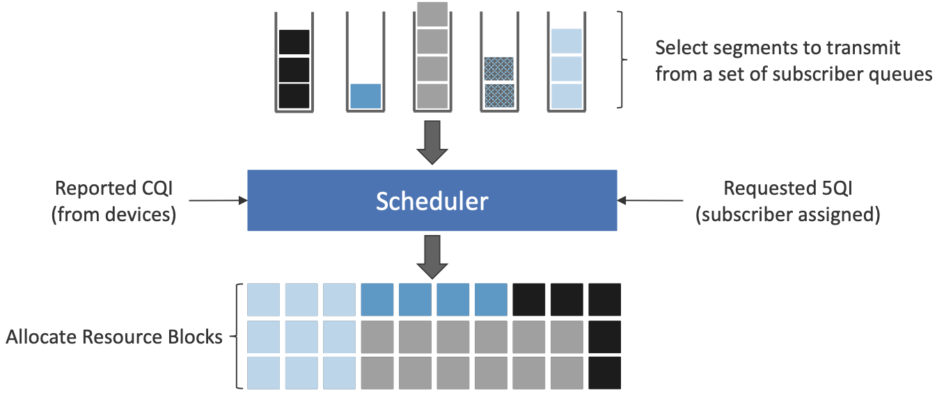
Figure 21. Scheduler allocates Resource Blocks to user data streams based on CQI feedback from receivers and the 5QI parameters associated with each class of service.

3.3 Virtualized Scheduler (Slicing)

The discussion up to this point presumes a single scheduler is suitable for all workloads, but different applications have different requirements for how their traffic gets scheduled. For example, some applications care about latency and others care more about bandwidth.

While in principle one could define a sophisticated scheduler that takes dozens of different factors into account, 5G has introduced a mechanism that allows the underlying resources (in this case radio spectrum) to be “sliced” between different uses. The key to slicing is to add a layer of indirection between the scheduler and the physical resource blocks. Slicing, like much of 5G, has received a degree of hype, but it boils down to virtualization at the level of the radio scheduler.

As shown in Figure 22, the idea is to first schedule offered traffic demands to virtual RBs, and then perform a second mapping of Virtual RBs to Physical RBs. This sort of virtualization is common in resource allocators throughout computing systems because we want to separate how many resources are allocated to each user (or virtual machine in the computing case) from the decision as to which physical resources are actually assigned. This virtual-to-physical mapping is performed by a layer typically known as a Hypervisor, and the important thing to keep in mind is that it is totally agnostic about which user’s segment is affected by each translation.

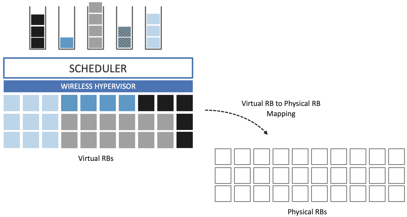
Figure 22. Wireless Hypervisor mapping virtual resource blocks to physical resource blocks.

Having decoupled the Virtual RBs from Physical RBs, it is now possible to define multiple Virtual RB sets (of varying sizes), each with its own scheduler. Figure 23 gives an example with two equal-sized RB sets. The important consequence is this: having made the macro-decision that the Physical RBs are divided into two equal partitions, the scheduler associated with each partition is free to allocate Virtual RBs independently from the other. For example, one scheduler might be designed to deal with high-bandwidth video traffic and another scheduler might be optimized for low-latency IoT traffic. Alternatively, a certain fraction of the available capacity could be reserved for premium customers or other high-priority traffic (e.g., public safety), with the rest shared among everyone else.

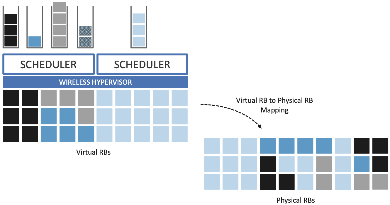
Figure 23. Multiple schedulers running on top of wireless hypervisor.

A final point to note is that there is considerable flexibility in the allocation of resources to slices. While the example above shows resources allocated in a fixed manner to each slice, it is possible to make unused resources in one slice available to another slice, as long as they can be reclaimed when needed. This is similar to how work-conserving scheduling works in network queues: resources are not wasted if the offered load in a class is less than the rate guaranteed for that class.

3.4 New Use Cases

We conclude by noting that up to this point we have described 5G as introducing additional degrees of freedom into how data is scheduled for transmission, but when taken as a whole, the end result is a qualitatively more powerful radio. This new 5G air interface specification, which is commonly referred to as New Radio (NR), enables new use cases that go well beyond simply delivering increased bandwidth. 3GPP defined five such use cases:

• Enhanced Mobile Broadband (eMBB)

• Ultra-Reliable Low-Latency Communications (URLLC)

• Massive Internet of Things (MIoT)

• Vehicle to Infrastructure/Vehicle (V2X)

• High-Performance Machine-Type Communications (HMTC)

These use cases reflect the requirements introduced in Chapter 1, and can be attributed to four fundamental improvements in how 5G multiplexes data onto the radio spectrum.

The first improvement is being able to change the waveform. This effectively introduces the ability to dynamically change the size and number of schedulable resource units, which opens the door to making fine-grained scheduling decisions that are critical to predictable, low-latency communication.

The second is related to the “Multiple Access” aspect of how distinct traffic sources are multiplexed onto the available spectrum. In 4G, multiplexing happens in both the frequency and time domains for downstream traffic, but only in the frequency domain for upstream traffic. 5G NR multiplexes both upstream and downstream traffic in both the time and frequency domains. Doing so provides finer-grained scheduling control needed by latency-sensitive applications.

The third advance is related to the new spectrum available to 5G NR, with the mmWave allocations opening above 24 GHz being especially important. This is not only because of the abundance of capacity—which makes it possible to set aside dedicated capacity for applications that require low-latency communication—but also because the higher frequency enables even finer-grained resource blocks (e.g., scheduling intervals as short as 0.125 ms). Again, this improves scheduling granularity to the benefit of applications that cannot tolerate unpredictable latency.

The fourth is related to delivering mobile connectivity to a massive number of IoT devices, ranging from devices that require mobility support and modest data rates (e.g. wearables, asset trackers) to devices that support intermittent transmission of a few bytes of data (e.g., sensors, meters). None of these devices are particularly latency-sensitive or bandwidth-hungry, but they often require long battery lifetimes, and hence, reduced hardware complexity that draws less power.

Support for IoT device connectivity revolves around allocating some of the available radio spectrum to a light-weight (simplified) air interface. This approach started with Release 13 of LTE via two complementary technologies: mMTC and NB-IoT (NarrowBand-IoT). Both technologies build on a significantly simplified version of LTE—i.e., limiting the numerology and flexibility needed to achieve high spectrum utilization—so as to allow for simpler IoT hardware design. mMTC delivers up to 1 Mbps over 1.4 MHz of bandwidth and NB-IoT delivers a few tens of kbps over 200 kHz of bandwidth; hence the term NarrowBand. Both technologies have been designed to support over 1 million devices per square kilometer. With Release 16, both technologies can be operated in-band with 5G, but still based on LTE numerology. Starting with Release 17, a simpler version of 5G NR, called NR-Light, will be introduced as the evolution of mMTC. NR-Light is expected to scale the device density even further.

As a complement to these four improvements, 5G NR is designed to support partitioning the available bandwidth, with different partitions dynamically allocated to different classes of traffic (e.g., high-bandwidth, low-latency, and low-complexity). This is the essence of slicing, as discussed above. Moreover, once traffic with different requirements can be served by different slices, 5G NR’s approach to multiplexing is general enough to support varied scheduling decisions for those slices, each tailored for the target traffic. We return to the applications of slicing in Chapter 6.